Classical Architectures in CNN

Since we have addressed the process of main building blocks in convolutional neural networks (CNN), now let’s take a look at several classical and modern CNN architectures. In this post, we will mainly focus on the classical architectures such as LeNet-5, AlexNet and VGG16 while modern network architectures such as Inception and ResNet will be introduced in the following posts.

LeNet-5

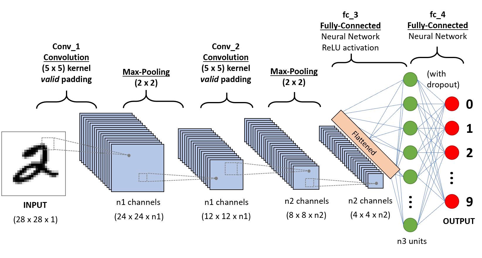
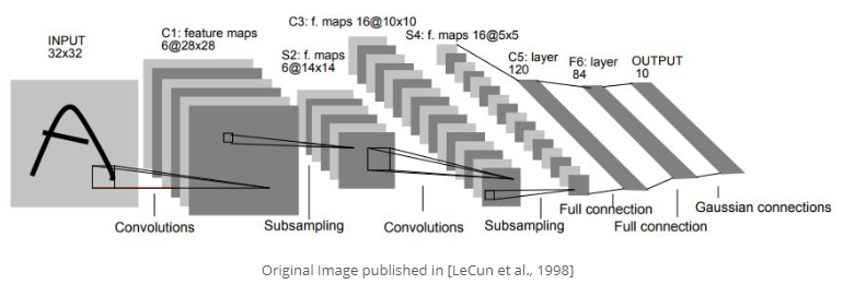
LeNet-5, a classical convolutional neural network that was introduced back to 1998, is aimed to recognize the digits from 0 to 9. The first figure below is the model architecture from the paper and the second one is the model that is similar to LeNet-5. LeNet-5 is such a classical model that it consists of two convolution layers followed by average pooling layers for each and apply three fully connected layers in the end of the network. The second model is quite similar to LeNet-5 except using max pooling layers.

LeNet-5

LeNet-5 modified version

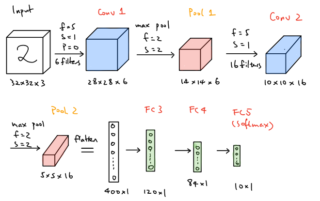
As shown above for the LeNet-5 modified model, the network takes a \(32\times32\times3\) image as the input and convolve it with 6 \(5\times5\times3\) filters and stride of 1, which results in a \(28\times28\times6\) output and then apply the output to a max pooling layer with the filter size of \(2\times2\) and stride of 2, which leads to a \(14\times14\times6\) output. Then apply the same convolution and max pooling layer again to obtain a \(5\times5\times16\) output. At the end of the network, the \(5\times5\times16\) output is flattened to a vector with the size of \(400\times1\) and then apply two fully connected layers to it and finally achieve the estimated output with the size of \(10\times1\) by using softmax.

Take the second architecture as an example, let’s practice how to compute the amounts of the parameters that are needed to learn in each layer of the network.

	Activation Size	Number of Parameters
Input	(32,32,3)	\(0\)
CONV1 (f=5, s=1, #6 filters)	(28,28,6)	\((5\times5\times3+1^{[b]})\times6=456\)
POOL1 (f=2, s=2)	(14,14,6)	\(0\)
CONV2 (f=5, s=1, #16 filters)	(10,10,16)	\((5\times5\times6+1^{[b]})\times16=2416\)
POOL2 (f=2, s=2)	(5,5,16)	\(0\)
FC3 (120 neurons)	(120,1)	\(5\times5\times16\times120+120^{[b]}=48120\)
FC4 (84 neurons)	(84,1)	\(120\times84+84^{[b]}=10164\)
FC5 (10 neurons)	(10,1)	\(84\times10+10^{[b]}=850\)

where b=bias and note that in the LeNet-5 network, they applied non-linearity activation function of sigmoid after each max pooling layer. In summary, the total number of parameters that the network needs to learn is approximately 62,000. According to this classical architecture, there are actually several patterns that the modern architectures still apply, which are the general structures of the networks - CONV –> POOL –> CONV –> POOL –> FC –> FC. That is, convolution layers are followed by pooling layers and a few of fully connected layers are located in the end of the network. Additionally, the trends of nowadays networks that \(n_H\) and \(n_W\) decrease while \(n_C\) increases as the networks go deeper are still applying.

AlexNet

AlexNet, introduced in 2012, employs an 8-layer convolutional neural network where the architecture is quite similar to LeNet-5, but there are also some significant differences. First, AlexNet is much deeper since it consists of five convolution layers, two hidden fully-connected layers and one fully-connected output layer as shown in the figure below. Aside from that, AlexNet used the ReLu activation function instead of sigmoid and the ReLu activation is processed after each convolution layer. Furthermore, dropout is also used after each fully connected layer except the output layer.

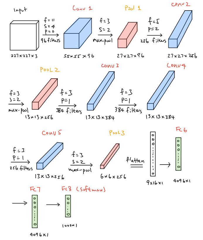
In the first layer of AlexNet, the convolution window size is \(11\times11\times3\). This is because this model is implemented to classify the inputs from ImageNet, the dataset which has bigger size. Consequently, a larger convolution window is applied in the first layer in order to capture the object. The brief structure of AlexNet can be illustrated as CONV–>POOL–>CONV–>POOL–>CONV–>CONV->CONV–>POOL–>FC–>FC–>FC. Notice that all convolutional layers in AlexNet apply the same padding and as the network goes deeper, more filters are used to convolve while the height and width of the activation shape are smaller. Furthermore, dropout is used after each fully connected layer in order to address the overfitting.

The amounts of the parameters that are needed to learn in each layer of the network is demonstrated below:

Layers	Activation Size	Numbers of Parameters
Input	\((227,227,3)\)	\(0\)
CONV1(f=11,s=4,p=0,96 filters)	\((55,55,96)\)	\((11\times11\times3+1)\times96=34,944\)
POOL1(f=3,s=2)	\((27,27,96)\)	\(0\)
CONV2(f=5,s=1,p=2,256 filters)	\((27,27,256)\)	\((5\times5\times96+1)\times256=614,656\)
POOL2(f=3,s=2)	\((13,13,256)\)	\(0\)
CONV3(f=3,s=1,p=1,384 filters)	\((13,13,384)\)	\((3\times3\times256+1)\times384=885,120\)
CONV4(f=3,s=1,p=1,384 filters)	\((13,13,384)\)	\((3\times3\times384+1)\times384=1,327,488\)
CONV5(f=3,s=1,p=1,256 filters)	\((13,13,256)\)	\((3\times3\times384+1)\times256=884,992\)
POOL3(f=3,s=2)	\((6,6,256)\)	\(0\)
FC6(4096 neurons)	\((4096,1)\)	\(6\times6\times256\times4096+4096=37,752,832\)
FC7(4096 neurons)	\((4096,1)\)	\(4096\times4096+4096=16,781,312\)
FC8(1000 neurons)	\((1000,1)\)	\(4096\times1000+1000=4,097,000\)

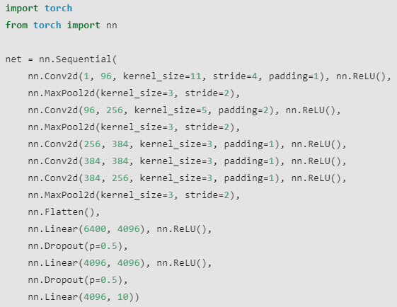
The total number of parameters needed to learn in AlexNet is approximately 60 million, which are way larger than LeNet-5 are. The Pytorch version code of AlexNet is illustrated below

VGG-16

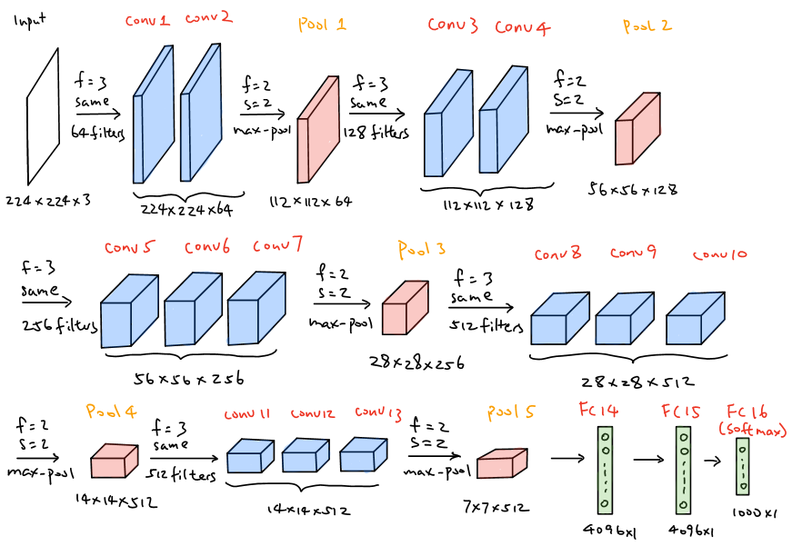
VGG-16, introduced in 2014, employs a 16-layer network, which is much deeper than AlexNet but offers a simpler network by replacing large kernel-size filters with multiple \(3\times3\) kernel-sized filters one after another. Aside from that, VGG-16 focuses on possibly simpler network where all the convolutional layer’s filter size are \(3\times3\) with stride of 1 and same padding whereas the max pooling layers all apply \(2\times2\) filter and stride of 2. The brief summary of VGG-16 is illustrated below.

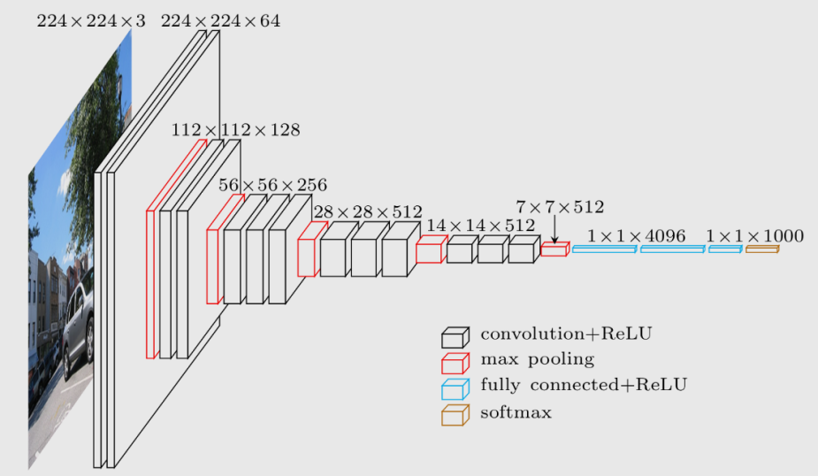
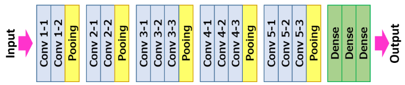
The patterns of VGG-16 are quite uniform that the network takes \(224\times224\times3\) image as the input, followed by a stack of two and three convolutional layers and ReLu activation function, then reduce the height and width by using pooling layer. For the number of filters in each convolutional layer, they are 64, 128, 256, 512 and 512, where as the network goes deeper the number of filters double in each stack of convolutional layer. Overall, there are approximately 138 million parameters needed to learn. Another phenomena that the modern networks also apply is that as the network goes deeper, \(n_H,n_W\) decrease due to the pooling layers and \(n_C\) increases due to the increasing number of filters in convolutional layers.