Pooling Layers
Pooling layer is another building blocks in the convolutional neural networks. Before we address the topic of the pooling layers, let’s take a look at a simple example of the convolutional neural network so as to summarize what has been done.
A Simple ConvNet Example
Suppose there is a \(39\times39\times3\) input image and then apply it to three convolution layers with following steps:
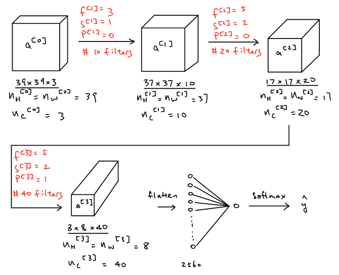
As shown in the figure above, the input layer \(a^{[0]}\) is convolved with 10 filters with size of \(3\times3\times3\), stride of 1 and without padding. The output size of the first convolution layer thus will be \(37\times37\times10\) where \(n_H^{[1]}=n_W^{[1]}=\lfloor\dfrac{39+0-3}{1}+1\rfloor=37\) and \(n_c^{[1]}=n_f=10\). Then, the output of the first convolution layer, as the input of the second convolution layer, is convolved with 20 filters with the size of \(5\times5\times10\), stride of 2 and without padding. The output size of the second convolutional layer thus will be \(17\times17\times20\) where \(n_H^{[2]}=n_W^{[2]}=\lfloor\dfrac{37+0-5}{2}+1\rfloor=17\) and \(n_c^{[2]}=n_f=20\). Then, the output of the second convolution layer, as the input of the third convolution layer, is convolved with 40 filters with the size of \(5\times5\times20\), stride of 2 and padding of 1. The output size of the third convolutional layer thus will be \(8\times8\times40\) where \(n_H^{[3]}=n_W^{[3]}=\lfloor\dfrac{17+2\times1-5}{2}+1\rfloor=8\) and \(n_c^{[3]}=n_f=40\). Then flattening all the neurons in the output of the third convolution layer and vectorize those neurons in order to form a vector with the size of \(2560\times1\) and finally apply softmax to obtain the value of \(\hat{y}\) in order to achieve the purpose of the tasks such as classification and etc.
Pooling Layers
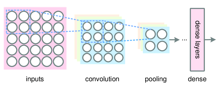
In general, there are three types of layer in a convolutional neural network, which are convolution layer (CONV), pooling layer (POOL) and fully connected layer (FC). Typically, several convolution layers are followed by a pooling layer and a few fully connected layers are at the end of the convolutional network.
The function of pooling layer is to reduce the spatial size of the representation so as to reduce the amount of parameters and computation in the network and it operates on each feature map (channels) independently. There are two types of pooling layers, which are max pooling and average pooling. However, max pooling is the one that is commonly used while average pooling is rarely used. The reason why max pooling layers work so well in convolutional networks is that it helps the networks detect the features more efficiently after down-sampling an input representation and it helps over-fitting by providing an abstracted form of the representation.
Max Pooling
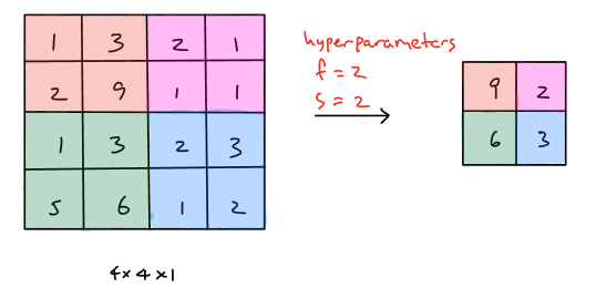
The operations of the max pooling is quite simple since there are only two hyperparameters used, which are filter size \((f)\) and stride \((s)\). Notice that we usually assume there is no padding in pooling layers, that is \(p=0\). Then we will illustrate two max pooling examples where \(f=2,s=2\) and \(f=3,s=1\) to demonstrate the process of the max pooling.
Example 1 (\(f=2,s=2\)):
Example 2 (\(f=3,s=1\)):
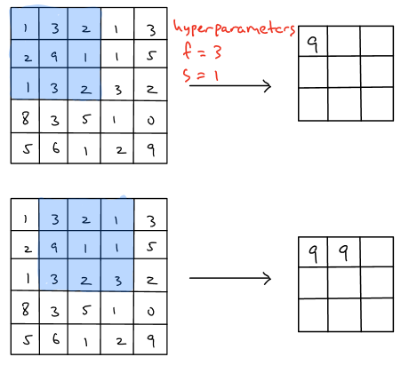
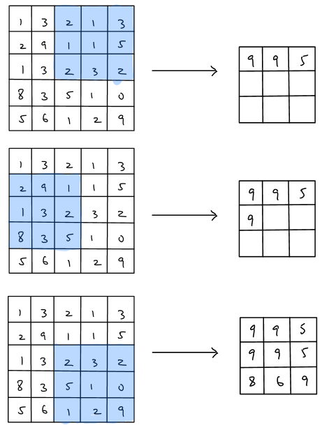
As shown in the figure above, it is important to realize that there is no parameters needed to learn in max pooling layer and furthermore it helps the overall network reduce the amount of parameters needed to learn, which save the computation cost of the network because the max pooling layer reduces \(n_H, n_W\) but not \(n_c\).
In summary, since there are only two hyperparameters in pooling layers, filter size \(f\) and stride \(s\), the size of the pooling layer input is \(n_H\times n_W \times n_c\) while the size of the pooling layer output is \(\lfloor \dfrac{n_H-f}{s}+1\rfloor \times \lfloor \dfrac{n_W-f}{s}+1\rfloor \times n_c\).