
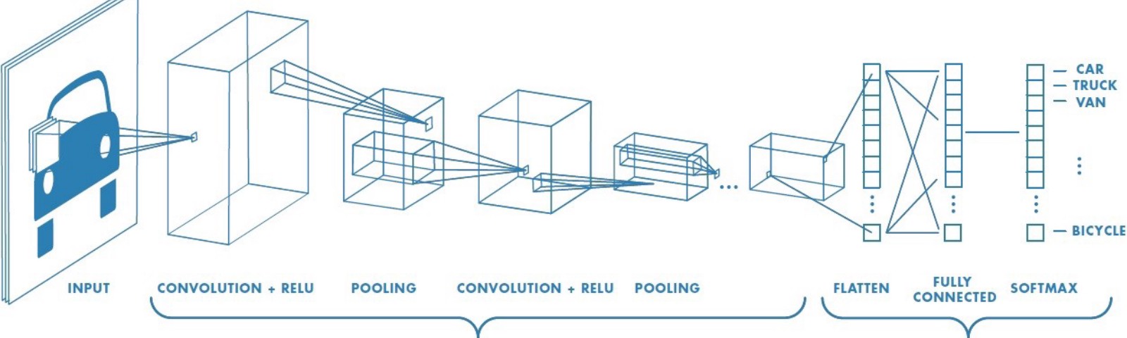
One Layer of a Convolutional Neural Networks
As mentioned in the last post, when we do the convolution operations, notice that the size of the input is \(n\times n\times c\) and the size of the filter is \(f\times f\times c\) where the channels of the input and the filter should be same. If there is only one filter, then the size of the generated output should be \((n-f+1)\times (n-f+1) \times 1\) (without padding and stride) while if there are \(n_f\) filters, then the size of the output will be \((n-f+1)\times (n-f+1) \times n_f\).
Convolutions Over Volume
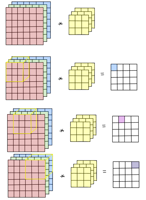
To figure out how it works in one specific layer of the convolutional neural network, we need to have a good command of how convolutions over volume works. For instance, if we have a \(6\times6\times3\) input image with 3 color channels (red, green and blue), to convolve with it, we need a filter with the size of \(f\times f\times 3\). Let \(f=3\). It is obvious that there are 27 numbers in the filter (9 numbers in each channel), the convolution operations are quite straightforward: select the specific region over each channel, multiply the corresponding entries and sum them up to achieve the value of each entry in the generated output. The procedures of the convolution over volume are illustrated below:
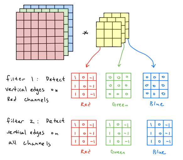
Notice that each filter could have different types of functions in order to obtain the feature map from the input image. For example, the first filter below is aimed to detect the vertical edges over red channels and the second filter is aimed to detect the vertical edges over all channels.
Multiple Filters
In practice, in one layer of the convolutional neural networks, there might have several types of filters with different purposes of feature extractions, thus we need to figure out how it works for multiple filters in convolutional neural networks. As we mentioned above, a \(n\times n\times c\) input image is convolved with \(n_f\) numbers of \(f\times f\times c\) filters, then the generated output size should be \((n-f+1)\times (n-f+1)\times n_f\). An simple example below is demonstrated:
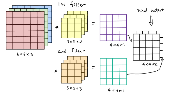
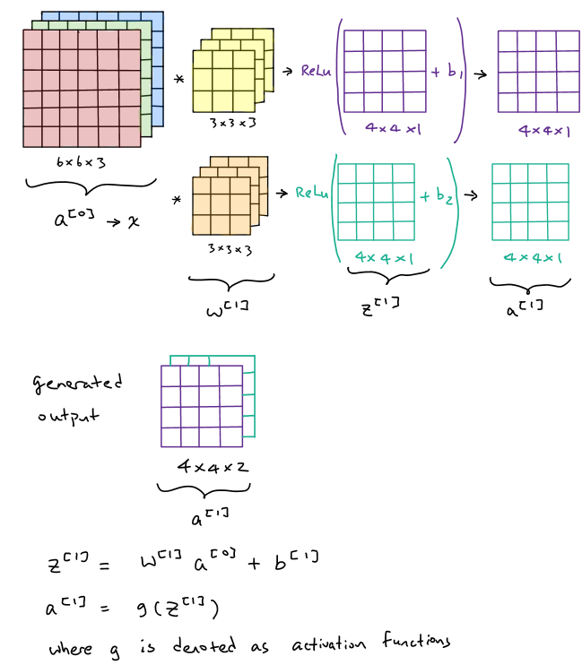
Typically, a complete layer of the convolutional neural network consists of the convolutions over volume operations and activation functions. To continue the previous example, after finishing the convolution operations over all color channels, we need to add a bias term and then apply a nonlinear activation function afterward, suppose it is a ReLu activation function. To complete, those two generated output has to be stacked together to obtain a \(4\times4\times2\) final output.
Denote the input image as \(a^{[0]}\) or \(x\). Then we could treat two filters as weight matrix \(w^{[1]}\) since the convolution operations here are actually conducting linear operations (simply multiply the entries and sum them up together). Denote \(z^{[1]}=w^{[1]}a^{[0]}+b^{[1]}\) and then output would be \(a^{[1]}=g(z^{[1]})\) where \(g\) is the activation function.
Summary of Notations
Continuing the example above, the summary of notation in one layer of the convolutional neural networks will be addressed below.
Denote:
\(f^{[l]}=\) filter size
\(p^{[l]}=\) padding size
\(s^{[l]}=\) stride size
\(n_c^{[l-1]}=c=\) numbers of input channels
\(n_c^{[l]}=n_f=\) numbers of filters \(=\) numbers of the output channels
\(a^{[l-1]}=n_H^{[l-1]}\times n_W^{[l-1]}\times n_c^{[l-1]}=n_H^{[l-1]}\times n_W^{[l-1]}\times c=\) input size
\(f^{[l]}\times f^{[l]} \times n_c^{[l-1]}=f^{[l]}\times f^{[l]} \times c=\) each filter size
\(a^{[l]}=n_H^{[l]}\times n_W^{[l]}\times n_c^{[l]}=n_H^{[l]}\times n_W^{[l]}\times n_f=\) output size
where input size \(n_H^{[l-1]},n_W^{[l-1]},n_c^{[l-1]}\) are known and
\(n_H^{[l]}=\lfloor \dfrac{n_H^{[l-1]}+2p^{[l]}-f^{[l]}}{s^{[l]}}+1\rfloor\), \(n_W^{[l]}=\lfloor \dfrac{n_W^{[l-1]}+2p^{[l]}-f^{[l]}}{s^{[l]}}+1\rfloor\), \(n_c^{[l]}=n_f\).
Furthermore, the single activation size is \(a^{[l]}=n_H^{[l]}\times n_W^{[l]}\times n_c^{[l]}\) and the overall activation size is \(A^{[l]}=n_H^{[l]}\times n_W^{[l]}\times n_c^{[l]}\times m\) where \(m\) is the numbers of the samples. The weight size is \(f^{[l]}\times f^{[l]} \times n_c^{[l-1]}\times n_c^{[l]}\) where \(n_c^{[l]}=n_f\) and bias\(=n_c^{[l]}=n_f=\) numbers of filters.