K-Nearest-Neighbor (KNN) Classification

Nearest Neighbor Classifier

K nearest neighbor classifier is rarely used in practice. But it allow us to get an idea about the basic approach to an classification problem.

• Dataset used: CIFAR-10
• Metrics used: L1 distance, L2 Euclidean distance
• Algorithm descriptions
  • Training: basically we just let computers memorize all the training images and test images.
  • Predicting: in predicting process, we use one of the metrics mentioned above and calculate the distance (L1 or L2) between each testing image and training image. Once we find the minimum distance between training image \(x_i\) and testing image \(y_j\), then we can assign corresponding labels that \(x_i\) has to the testing image \(y_i\). For example, if the first testing image, \(y_1\), has the minimum distance to training image, \(x_{49920}\) among all 50000 training images. Then we assign the label of \(x_{49920}\), suppose it is class 6, to the testing image, \(y_1\). That is the class of \(y_1\) would be class 6. So on so far, we iterate this process for all testing images.
  • But the algorithm accuracy turns out not so good. Only around 3 out of 10 images can predict correctly.

Different K values

the algorithm above describes that we can find the minimum distance from testing images to training images and then assign the labels of the corresponding training image, \(x_i\) to the testing image, \(y_j\). This is the representation of how Nearest Neighbor works in which \(k=1\).

However, we could choose different values for \(k\), and it turns out \(k=1\) does not always perform as well as some other values of \(k\).

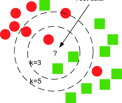
The way how kNN works is, for instance, you have a distance vector for one individual testing image, \(y_1\), then the distance vector would be the form of \(R^{50000}\), each entry in the vector represents the corresponding distance from testing image, \(y_1\), to each training image, \(x_i\), where \(i=1,2,..,50000\). Then, you select the value of \(k\), which represents that you find the number of \(k\) smallest or closest distance from testing image, \(y_1\), to each training images, \(x_i\).

For instance, if you choose \(k=5\), and there are 3 data points are belonged to class 10 while the other 2 data points are belonged to class 2. Consequently, you will classify the testing image, \(y_j\), into the class 10. Intuitively, higher values of \(k\) have a smoothing effect that makes the classifier more resistant to the outliers.

Validation

Aforementioned above, different value \(k\) leads to different classifiers. But what value of \(k\) should we use? It leads to the topics of validation. Additionally, you saw many different functions we could have used: L1 norm, L2 norm and some other metrics such as dot product. These choices of metrics are called hyperparameter. It is often not obvious what values/setting one should choose.

In this CIFAR-10 KNN case, we could choose different value of \(k\), and different metrics to fit the testing images in order to reach a better accuracy. However, this is not always the case because in practice, we cannot use the testing dataset for the purpose of tweaking hyperparameters. In other word, the testing data is the precious resource that should be never touched until the end. Once you do use the testing data for getting a better hyperparameter, it is called overfit because you actually treat the testing data as part of your training data. Even though it worked well for this testing data, most of time it would perform very bad if you deploy the model to other dataset. Therefore, the purpose of avoiding testing data applied in your algorithm is to remain a good proxy for measuring the generalization of your classifier.

Indeed, it does have a correct way of tuning the hyperparameters without touching the testing data at all. The idea behind it is to split your training data in two: a slightly smaller training set, which is called validation set. Using CIFAR-10 as an example, we could use 49,000 of the training images for training and 1,000 of it for validation.

Cross-validation

There is another more sophisticated technique for hyperparameter tuning, which is called cross-validation. The idea behind is that instead of arbitrarily picking 1,000 training images as validation set, you could split the training data into 5 equal folds and use 4 out of 5 folders for training and the other subfolder as validation set. We could iterate over which folder is the validation set, evaluate the performance and finally average the performance across different folders. But this does require a lot of computations involved and it is not commonly used methods for validation in practice.