Softmax Function and Cross Entropy Loss Function

There are many types of loss functions as mentioned before. We have discussed SVM loss function, in this post, we are going through another one of the most commonly used loss function, Softmax function.

Definition

The Softmax regression is a form of logistic regression that normalizes an input value into a vector of values that follows a probability distribution whose total sums up to 1. As its name suggests, softmax function is a “soft” version of max function. Instead of selecting one maximal value such as SVM, softmax function breaks the whole (sum to 1) into different elements with probability, maximal element getting the largest portion of the distribution while other smaller elements getting relatively small value of it as well. This property of softmax function which generates a probability distribution makes it suitable for probabilistic interpretation in classification tasks. Softmax function is defined as below:

\[P(y_i|x_i;W)=\dfrac{e^{f_{y_i}}}{\sum_je^{f_{j}}}\]

It can be interpreted as the probability assigned to the correct label \(y_i\) given the training image, \(x_i\) parameterized by \(W\). Furthermore, the score function \(f(x_i;W)\) stays the same as SVM describes before. That is \(f(x_i;W)=Wx_i\). Instead of comparing each element in \(f(x_i;W)\) and return the max value between obtained score and 0, in softmax function, you take the exponential value of the correct class score, \(f_{y_i}\) and then sum up all the exponential value of the scores for each class, which is \(f_j\), the \(j\)-th element of the score vector \(Wx_i\) for image \(x_i\).

Unnormalized softmax function

def softmax_unnormalized(f):
    '''
    input f is a numpy array

    '''
    prob = np.exp(f)/np.sum(np.exp(f))
    return prob

The method described above is unnormalized softmax function, which is not good sometimes. For example, the exponential value of a big value such as 1000 almost goes to infinity, which cause the program returns ‘nan’.

f = np.array([100, 400, 800])
p = softmax_unnormalized(f)

>>>p
array([ 0.,  0., nan])

Normalized/Standard softmax function

In order to prevent this kind of numerical typos, we could normalize the input and avoid of having big values. To do so, you can substract the maximum value among the array from the entire array, which is demonstrated below:

def softmax_standard(f):
    '''
    input f is a numpy array

    '''
    f = f - np.max(f)
    prob = np.exp(f)/np.sum(np.exp(f))
    return prob

Again, the original input is \([100,400,800]\). After normalization, the vector becomes \([-700,-400,0]\), which avoids the occurrence of ‘nan’​.

f = np.array([100, 400, 800])
p = softmax_standard(f)

>>>p
array([9.85967654e-305, 1.91516960e-174, 1.00000000e+000])

Cross-entropy loss function

Now, we have computed the score vectors for each image \(x_i\) and have implemented the softmax function to somehow transform the numerical scores to probability distribution. Compared to other classes, the probability of the correct class is supposed to be close to 1 for a better classification. The next thing we want to consider is how to correlate the computed probability distribution with the loss function.

Interpretation of softmax function and cross-entropy loss function

since the softmax function is defined as follow:

\[P(y_i|x_i;W)=\dfrac{e^{f_{y_i}}}{\sum_je^{f_{j}}}\]

It can be interpreted as the probability of the correct class \(y_i\) given the image \(x_i\), and we want it to be close to 1, meaning we classify this image to its correct class.

At the same time, we want the loss for the correct class to be 0. Intuitively, if we classify the image to its correct class, then the corresponding loss for this image is supposed to be 0

To correlate with the probability distribution and the loss function, we can apply log function as our loss function because log(1)=0, the plot of log function is shown below:

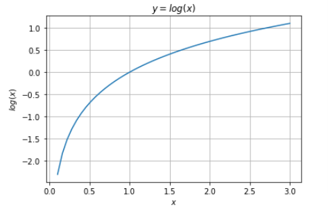
Here, considered the other probability of incorrect classes, they are all between 0 and 1. Taking the log of them will lead those probabilities to be negative values. To avoid that, we need to add a ‘minus’ sign when we take log because the minimum loss is 0 and cannot be negative. Hence, it leads us to the cross-entropy loss function for softmax function.

Cross-entropy loss function for softmax function

The mapping function \(f:f(x_i;W)=Wx_i\) stays unchanged, but we now interpret these scores as the unnormalized log probabilities for each class and we could replace the hinge loss/SVM loss with a cross-entropy loss that has the form:

\[\begin{align*} L_i&=-log(P(y_i|x_i;W))\\ &=-log(\dfrac{e^{f_{y_i}}}{\sum_je^{f_{j}}})\\ &=-log(e^{f_{y_i}})+log(\sum_je^{f_{j}})\\ &=-f_{y_i}+log(\sum_je^{f_{j}}) \end{align*}\]

where \(f_{y_i}\) is the probability for correct class score and \(f_j\) is the \(j\)-th element of the score vector for each image.

To interpret the cross-entropy loss for a specific image, it is the negative log of the probability for the correct class that are computed in the softmax function.

def softmax_loss_vectorized(W, X, y, reg):

    """

    Softmax loss function --> cross-entropy loss function --> total loss function

    """

    # Initialize the loss and gradient to zero.
    loss = 0.0
    num_classes = W.shape[1]
    num_train = X.shape[0]

    # Step 1: compute score vector for each class
    scores = X.dot(W)

    # Step 2: normalize score vector, letting the maximum value to 0
    scores = scores- scores.max()
    scores = np.exp(scores)

    #Step 3: obtain the correct class score
    correct_score = scores[range(num_train), y]
    #compute the sum of exp of all scores for all classes
    scores_sums = np.sum(scores, axis=1)

    #Step 4: compute softmax function
    softmax_loss = correct_score / scores_sums
    #compute cross-entropy function
    cross_entropy_loss = - np.log(softmax_loss)
    #compute loss function
    loss = np.sum(cross_entropy_loss)/num_train

    return loss