Logistic Regression

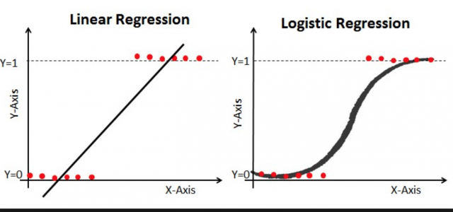
Logistic regression is a technique in machine learning and is used to deal with the binary classification problem in supervised learning where the output of this type of problem has two-class value, i.e either 0 or 1. It is named for the function it used, which is logistic function or sigmoid function.

Consider a binary classification problem, given the input \(x\), we want the estimated output that indicates which class the input is. Generally, we could estimate the probability of the output to between 0 or 1 and then set up a threshold that can help us decide its estimated class, which is also the estimated output. Therefore, denote the probability of the estimated output as \(\hat{y}\) and let \(\hat{y} = p(y\|x)\). Obviously, the value of \(\hat{y}\) is supposed to be between 0 and 1, i.e. \(0 \le \hat{y} \le 1\). On the other hand, our hypothesis model is \(z=wx+b\) so as to estimate the output by using parameters weight \(w\) and bias \(b\) where \(w\in R^n, b\in R\). Clearly the value of \(z\) is not the probability of chance that is between 0 and 1. Therefore, in order to generate the output in the form of probability, we need transform \(z\) to \(\hat{y}\) by using the logistic function or sigmoid function.

Logistic/Sigmoid Function

Instead of fitting a straight line or hyperplane, the logistic regression model uses the logistic function to squeeze the output of a linear operation equation between 0 and 1. It is defined as below:

\[\sigma(z)=\dfrac{1}{1+e^{-z}}\]

where \(\sigma(.)\) is the logistic function notation.

The graph of sigmoid function is illustrated below:

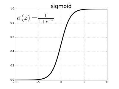
When \(z\) is positively large, the value of \(\sigma(z)\) converges to 1 while \(z\) is negatively small, the value of \(\sigma(z)\) converges to 0.

To summarize, the model that logistic regression uses is that given the input \(\{x^{(1)},...,x^{(m)}\}\) and corresponding outputs \(\{y^{(1)},...,y^{(m)}\}\), we have the estimated output probability \(\hat{y}^{(i)}=\sigma(w^Tx^{(i)}+b)\) where \(\sigma(z)=\dfrac{1}{1+e^{-z}}\) and by setting up the threshold, we want the estimated output probability \(\hat{y}^{(i)}\) greater than the threshold so that it can be assigned to the class where \(y^{(i)}\) actually belongs to. Notice that \(y^{(i)}\in\{ 0,1\}\) and \(\hat{y}^{(i)}\) is between 0 and 1. For instance, by setting up an threshold of 0.5, any estimated output probability, \(p(y=1\|x)\), that is greater than 0.5, then we will assign the class of 1, otherwise, it will be assigned to the class of 0.

Logistic Regression Cost Function

Unlike the cost function in linear regression, logistic regression does not apply the mean square error as its cost function since it will become a non-convex function, which is impossible to find the global minimum. In order to be a convex function and reach the global minimum when conducting the gradient descent, instead, the loss function for a single sample in the training dataset that the logistic regression applies is shown below:

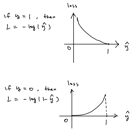
\[L(\hat{y}^{(i)},y^{(i)})=-[y^{(i)}~log(\hat{y}^{(i)})+(1-y^{(i)})log(1-\hat{y}^{(i)})]\]

If \(y=1\), the loss function becomes \(L(\hat{y}^{(i)},y^{(i)})=-log(\hat{y}^{(i)})\). Theoretically, We want the loss function as small as possible to predict relatively accurate outputs. Consequently, we want the term \(-log(\hat{y}^{(i)})\) as small as possible, but keep it in mind that the loss is always non-negative, that is, we want \(log(\hat{y}^{(i)})\) large and \(\hat{y}^{(i)}\) large as well. Another thing is that the value of \(\hat{y}\) is between 0 and 1; therefore, we want \(\hat{y}\) as close as to 1. In other words, the value of \(z\) is supposed to be as large as possible due to the relationship between \(z\) and \(\hat{y}\) aforementioned.

If \(y=0\), the loss function is \(L(\hat{y}^{(i)},y^{(i)})=-log(1-\hat{y}^{(i)})\), in order to make loss as small as possible, \(-log(1-\hat{y}^{(i)})\) needs to be small enough, that is, we want \(log(1-\hat{y}^{(i)})\) large and \(1-\hat{y}^{(i)}\) large as well, which leads to a small enough positive value of \(\hat{y}^{(i)}\) as close as to 0, which is also being said that the corresponding value \(z\) needs to be as negatively small as possible.

Another way to think about this is by considering the relationship between loss function and \(\hat{y}\) as shown below. Notice that the value of \(\hat{y}\) is always between 0 and 1. In the case when \(y=1\), the relationship between loss and \(\hat{y}\) is monotonically decreasing, thus in order to make loss small, we need \(\hat{y}\) close to 1 and corresponding \(z\) as positively large as possible. When \(y=0\), the relationship is monotonically increasing; therefore, we want \(\hat{y}\) close to 0 and corresponding value \(z\) as negatively small as possible.

Based on the loss function for a single sample in training dataset, the cost function in terms of the entire training dataset is defined as followed:

\[J(w,b)=\dfrac{1}{m} \sum_{i=1}^m L(\hat{y}^{(i)},y^{(i)})\\ where~L(\hat{y}^{(i)},y^{(i)})=-[y^{(i)}~log(y^{(i)})+(1-y^{(i)})log(1-\hat{y}^{(i)})]\\ and~\hat{y}^{(i)} = \sigma(w^Tx^{(i)}+b)~where~\sigma(z)=\dfrac{1}{1+e^{-z}}\]

Our goal is to minimize the cost function for the entire training samples in terms of the parameters \(w\) and \(b\). One of methods to minimize the cost function is gradient descent, which is aimed to find the global minimum by looking for the gradient of the cost function in terms of the specific parameters. We will address the topic of gradient descent in the next post.