Computational Graph and Backpropagation

In the previous post, we address the topics of gradient descent in order to minimize the loss function. Now we have to get familiar to computing the analytic gradient for arbitrarily complex function by using the framework of computational graphs. We can apply computational graph to represent any function with forward pass and backward pass so that we could use the computational graph to compute the gradient or derivative of the loss function with respect to the parameters.

Simple Example

Let’s start from a really simple example. Consider a loss function \(J\) parameterized by \(a,b,c\) where \(J(a,b,c)=3(a+bc)\). First, let’s start from the forward pass, which is quite simple. The forward pass refers to the regular computations that conduct the operations such as adding, subtracting, multiplying and etc in the direction from left to right. The only thing we need to notice is that we could divide the complex functions into single computation components and then combine them together to represent the whole function. Thus, denote \(u=bc\), \(v=a+u\) and \(J=3v\). The figure below illustrates how forward pass works for this function:

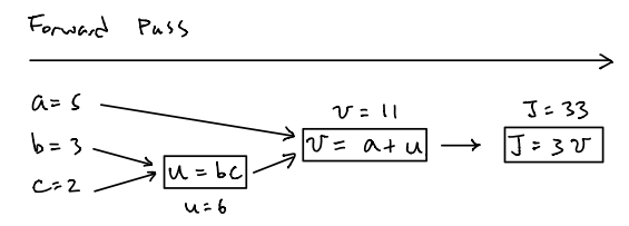
While for the backward pass or backpropagation, its ultimate goal is just to compute the gradient of the loss function with respect to parameters, which are \(\dfrac{dJ}{da},\dfrac{dJ}{db},\dfrac{dJ}{dc}\). To do so, we need to compute the gradient of all components in the direction from right to left. The figure below illustrates how backward pass works for this example:

First, we have to compute the gradient of \(\dfrac{dJ}{dv}\) on the most right hand side so as to be able to compute the gradient of \(\dfrac{dJ}{da}\) next since \(\dfrac{dJ}{da}=\dfrac{dJ}{dv}\dfrac{dv}{da}\) according to the chain rule. In other words, the value of \(\dfrac{dJ}{da}\) is determined by \(\dfrac{dJ}{dv}\), which is the gradient on its right hand side and this is also why we need to compute the gradient from right to left. To compute the gradients of \(\dfrac{dJ}{db}\) and \(\dfrac{dJ}{dc}\), we need to compute the gradient of \(\dfrac{dJ}{du}\) first due to the facts that \(\dfrac{dJ}{db}=\dfrac{dJ}{du}\dfrac{du}{db}\) and \(\dfrac{dJ}{dc}=\dfrac{dJ}{du}\dfrac{du}{dc}\).

Gradient for Logistic Regreession

Based on the previously simple example, let’s draw the computational graph and compute the gradient of loss function for logistic regression discussed in the last post. Suppose there are only two features \(x_1,x_2\) and thus \(x=\begin{bmatrix}x_1&x_2\\\end{bmatrix}^T\), \(w=\begin{bmatrix}w_1&w_2\\\end{bmatrix}^T\). Then, to compute the gradients of \(\dfrac{dL}{dw_1}\),\(\dfrac{dL}{dw_2}\) and \(\dfrac{dL}{db}\), we have three components in the computational graph, \(L(\hat{y},y)=-[y~log(\hat{y})+(1-y)log(1-\hat{y})]\), \(\hat{y}=\sigma(z)\) and \(z=wx+b\) or \(z=w_1x_1+w_2x_2+b\) in the direction from right to left.

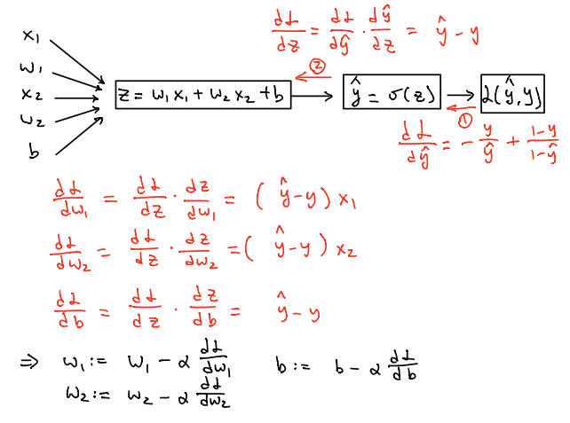
Therefore, we need to compute the gradient of \(\dfrac{dL}{d\hat{y}}\) on the most right hand side first. Based on the fact from basic calculus that \(\dfrac{d}{dx}log(x)=\dfrac{1}{x}\) and \(\dfrac{d}{dx}log(-x)=-\dfrac{1}{x}\), we know that:

\[\begin{align*} \dfrac{dL}{d\hat{y}}&=\dfrac{d}{d\hat{y}}[-y~log(\hat{y})-(1-y)log(1-\hat{y})] &=-\dfrac{y}{\hat{y}}+\dfrac{1-y}{1-\hat{y}} \end{align*}\]

Then in order to compute the gradient of \(\dfrac{dL}{dz}\) which can be inferred as \(\dfrac{dL}{dz}=\dfrac{dL}{d\hat{y}}\dfrac{d\hat{y}}{dz}\), we have to find out the gradient of \(\dfrac{d\hat{y}}{dz}\) first and the proof is shown below:

\[\begin{align*} \dfrac{d\hat{y}}{dz}&=\dfrac{d}{dz}(1+e^{-z})^{-1}\\ &=-(1+e^{-z})^{-2}(-e^{-z})\\ &=\dfrac{e^{-z}}{(1+e^{-z})^2}\\ &=(\dfrac{1}{1+e^{-z}})(\dfrac{e^{-z}}{1+e^{-z}})\\ &=(\dfrac{1}{1+e^{-z}})(\dfrac{1+e^{-z}-1}{1+e^{-z}})\\ &=(\dfrac{1}{1+e^{-z}})(1-\dfrac{1}{1+e^{-z}})\\ &=\hat{y}(1-\hat{y}) \end{align*}\]

Based on the above inference, we have

\[\begin{align*} \dfrac{dL}{dz}=\dfrac{dL}{d\hat{y}}\dfrac{d\hat{y}}{dz}&= (-\dfrac{y}{\hat{y}}+\dfrac{1-y}{1-\hat{y}})(\hat{y}(1-\hat{y}))\\ &=-y(1-\hat{y})+(1-y)\hat{y}\\ &=-y+y\hat{y}+\hat{y}-y\hat{y}\\ &=\hat{y}-y \end{align*}\]

Therefore, \(\dfrac{dL}{dz}=\hat{y}-y\). Our ultimate goal is to compute the gradients of \(\dfrac{dL}{dw_1}\),\(\dfrac{dL}{dw_2}\) and \(\dfrac{dL}{db}\). It is much simpler to compute those three gradients once we find out the value of \(\dfrac{dL}{dz}\) and thus we have

\[\dfrac{dL}{dw_1} = \dfrac{dL}{dz}\dfrac{dz}{dw_1} = (\hat{y}-y)x_1\\ \dfrac{dL}{dw_2} = \dfrac{dL}{dz}\dfrac{dz}{dw_2} = (\hat{y}-y)x_2\\ \dfrac{dL}{db} = \dfrac{dL}{dz}\dfrac{dz}{db} = \hat{y}-y\\\]

Then, on each iteration, we use the above equations to compute those gradients and update the parameters \(w_1,w_2,b\) by using the formulas \(w_1:=w_1-\alpha \dfrac{dL}{dw_1}\), \(w_2:=w_2-\alpha \dfrac{dL}{dw_2}\) and \(b:=b-\alpha \dfrac{dL}{db}\). However, this is just the updates for parameters in terms of single sample instead of the entire sample. Once the sample size is extremely large and if we use for loop to update the parameters for each sample, it will take tons of time, which is not a wise way to do so. Next, we will address how to vectorize the logistic regression in order to update the parameters quickly by vectorizing.

Vectorizing Logistic Regression

First of all, the thing we need to notice is that the logistic regression example for a single sample shown above is under the assumption that the dimension feature are two dimensions, that is \(x=\begin{bmatrix}x_1&x_2\\\end{bmatrix}^T\). Consequently, the formulas we have above are \(\dfrac{dL}{dw_1} = (\hat{y}-y)x_1\), \(\dfrac{dL}{dw_2}= (\hat{y}-y)x_2\). Suppose the feature dimensions are n-dimension, then the gradient formulas for \(\dfrac{dL}{dw_i}\) where \(i\in\{1,..,n\}\) is \(\dfrac{dL}{dw_i} = (\hat{y}-y)x_i\). To vectorize it, we have \(\dfrac{dL}{dw} = (\hat{y}-y)x\) where \(x=\begin{bmatrix}x_1&..&x_n\\\end{bmatrix}^T\) and \(w=\begin{bmatrix}w_1&..&w_n\\\end{bmatrix}^T\).

Therefore, for a single sample, we have inferred that \(\dfrac{dL}{dz}^{(j)}:=dz^{(j)}=\hat{y}^{(j)}-y^{(j)}\) and then \(\dfrac{dL}{dw}^{(j)}=(\hat{y}^{(j)}-y^{(j)})x^{j}\), \(\dfrac{dL}{db}^{(j)}=\hat{y}^{(j)}-y^{(j)}=dz^{(j)}\) where \(j\in\{1,...,m\}\) and \(m\) is the sample size. Now, if we compute the gradients over the entire sample, then the formula to compute \(\dfrac{dL}{db}\) is

\[\begin{align*} \dfrac{dL}{db}&=\dfrac{1}{m}[\hat{y}^{(1)}-y^{(1)}+...+\hat{y}^{(m)}-y^{(m)}]\\ &=\dfrac{1}{m}(dz^{(1)}+...+dz^{(m)}) \end{align*}\]

Thus, if we vectorize \(dz\) as \(dz=\begin{bmatrix}dz^{(1)}&..&dz^{(m)}\\\end{bmatrix}^T\), then the value of \(\dfrac{dL}{db}\) is the sum of all elements in the vector \(dz\) over \(m\).

On the other hand, to compute the gradient of \(\dfrac{dL}{dw}\), we have

\[\begin{align*} \dfrac{dL}{dw}&=\dfrac{1}{m}[(\hat{y}^{(1)}-y^{(1)})x^{(1)}+...+(\hat{y}^{(m)}-y^{(m)})x^{(m)}]\\ &=\dfrac{1}{m}(dz^{(1)}x^{(1)}+...+dz^{(m)}x^{(m)})\\ &=\dfrac{1}{m}\begin{bmatrix}x^{(1)}&..&x^{(m)}\\\end{bmatrix} \begin{bmatrix}dz^{(1)}&..&dz^{(m)}\\\end{bmatrix}^T\\ &=\dfrac{1}{m}Xdz^T \end{align*}\]

where \(X=\begin{bmatrix}x^{(1)}&..&x^{(m)}\\\end{bmatrix}\) and \(X\in R^{n\times m}\). Therefore, we can use the formula of \(\dfrac{dL}{dw}=\dfrac{1}{m}Xdz^T\) to compute the gradient of \(\dfrac{dL}{dw}\).

In summary, to compute the gradients and update the parameters of \(w,b\) on each iteration (suppose 100 iterations total), the vanilla code is illustrated below:

for iteration in range(100):
    z = np.dot(w.T, X) + b
    A = sigma(z)
    dz = A - Y
    dw = np.dot(X, dz.T) / m
    db = np.sum(dz) / m
    w -= alpha * dw
    b -= alpha * db