Neural Networks

Quick Introduction to Neural Networks

In the following posts, we will discuss the neural networks in machine learning and deep learning, which is one of the most important topics in those areas. Neural networks are modeled as collections of neurons that are connected in an acyclic graph. It can be multiple layers in neural networks and the outputs of one layer will be the inputs of the following layer. For regular neural networks, the most common layer type is the fully-connected layer where neurons between two adjacent layers are fully pairwise connected, but neurons within a single layer don’t share the connections. Below are two examples of fully-connected layer of neural networks:

The left figure illustrates a two-layer fully-connected neural network with one hidden layer and one output layer while the right one shows a three-layer fully-connected neural network with two hidden layers and one output layer.

One of the most important thing in neural networks is that each layer generally has an activation function except the output layer. This is because the last output layer is usually taken as real-valued numbers to represent the class scores (e.g. classification) or as real-valued target (e.g. regression). The reason why each layer has an activation function will be discussed below in the section of Activation Function.

The figure below demonstrates an example of two-layer neural networks notation.

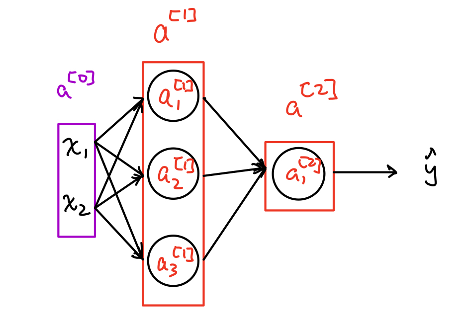
The input layer is denotes as \(a^{[0]}\) while the first hidden layer is denoted as \(a^{[1]}\) and it has three hidden units total. Each hidden unit is denoted as \(a_i^{[1]}\), represented as the \(i\)-th hidden unit in the 1st hidden layer. Additionally, we denote the vectorized first-hidden-layer as \(a^{[1]}\) and \(a^{[1]}=\begin{bmatrix}a_1^{[1]}&a_2^{[1]}&a_3^{[1]}\\\end{bmatrix}^T\).

Computing a Neural Network’s Output

After being familiar with the notation of neural networks, let’s discuss how to compute the final output through the hidden layers. Take the same neural network example above, we have a single sample input \(x=a^{[0]}=\begin{bmatrix}x_1&x_2\\\end{bmatrix}^T\) with the shape of (2,1).

The value of \(a_i^{[1]}\) is obtained by mapping the function of \(a_i^{[1]}=\sigma(z_i^{[1]})\) where \(\sigma(.)\) is the sigmoid activation function while the value of \(z_i^{[1]}\) is computed by the formula \(z_i^{[1]}={w_i^{[1]}}^T x+b_i^{[1]}\) where \(w_i^{[1]}\) is the weight with the shape of (2,1) and \(b_i^{[1]}\) is a real number bias term. Then, the exact value of \(a_i^{[1]}\) and \(z_i^{[1]}\) for the first hidden layer are computed by the following demonstration:

\[z_1^{[1]}={w_1^{[1]}}^T x+b_1^{[1]}, ~~a_1^{[1]}=\sigma(z_1^{[1]})\\ z_2^{[1]}={w_2^{[1]}}^T x+b_2^{[1]}, ~~a_2^{[1]}=\sigma(z_2^{[1]})\\ z_3^{[1]}={w_3^{[1]}}^T x+b_3^{[1]}, ~~a_3^{[1]}=\sigma(z_3^{[1]})\\\]

Now, to vectorize those three terms, we have

\[z^{[1]}=\begin{bmatrix}z_1^{[1]}\\z_2^{[1]}\\z_3^{[1]}\end{bmatrix}= \begin{bmatrix}-{w_1^{[1]}}^T-\\-{w_2^{[1]}}^T-\\-{w_3^{[1]}}^T-\end{bmatrix} \begin{bmatrix}x_1\\x_2\end{bmatrix} + \begin{bmatrix}b_1^{[1]}\\b_2^{[1]}\\b_3^{[1]}\end{bmatrix}\]

and

\[a^{[1]}=\begin{bmatrix}a_1^{[1]}\\a_2^{[1]}\\a_3^{[1]}\end{bmatrix}= \begin{bmatrix}\sigma(z_1^{[1]})\\\sigma(z_2^{[1]})\\\sigma(z_3^{[1]})\end{bmatrix}\]

While the values for the second hidden layer, \(z_i^{[1]}\) and \(a_i^{[1]}\) can be computed based on the formulas below:

\[z^{[2]} = \begin{bmatrix}z_1^{[2]}\end{bmatrix} = \begin{bmatrix}-{w_1^{[2]}}^T-\end{bmatrix}\begin{bmatrix}x_1\\x_2\end{bmatrix} + \begin{bmatrix}b_1^{[2]}\end{bmatrix}\]

and

\[a^{[2]}=\begin{bmatrix}a_1^{[2]}\end{bmatrix}= \begin{bmatrix}\sigma(z_1^{[2]})\end{bmatrix}\]

To summarize, we have the vectorized version of computation for the overall neural networks, which are

\[z^{[1]}=W^{[1]}a^{[0]}+b^{[1]}\\ a^{[1]}=\sigma(z^{[1]})\\ z^{[2]}=W^{[2]}a^{[1]}+b^{[2]}\\ a^{[2]}=\sigma(z^{[2]})\\\]

where \(a^{[0]}=x\) by denoting \(W^{[1]}=\begin{bmatrix}-{w_1^{[1]}}^T-\\-{w_2^{[1]}}^T-\\-{w_3^{[1]}}^T-\end{bmatrix}\) with the shape of (3,2) and \(b^{[1]}=\begin{bmatrix}b_1^{[1]}\\b_2^{[1]}\\b_3^{[1]}\end{bmatrix}\) with the shape of (3,1), which results in \(z^{[1]}\) with the shape of (3,1). On the other hand, \(W^{[2]}=\begin{bmatrix}-{w_1^{[2]}}^T-\end{bmatrix}\) with the shape of (1,3).

Vectorizing across Multiple Examples

What we discussed above is only in terms of the single training sample, now let’s address how to compute the output in terms of the entire samples. Suppose we have \(m\) training examples. Denote \(x^{(i)}\) as the \(i\)-th input example and \(z^{[1](i)}\) represents the \(i\)-th value of the first hidden layer before the activation function while \(a^{[1](i)}\) represents the \(i\)-th value of the first hidden layer after the activation function. Same interpretation for \(z^{[2](i)}\) and \(a^{[2](i)}\).

To compute the output across the entire samples, originally, we could have the following formula without vectorizing which are

for i in range(m):
    z_1_i = W_1 @ x_i + b_1
    a_1_i = sigmoid(z_1_i)
    z_2_i = W_2 @ a_1_i + b_2
    a_2_i = sigmoid(z_2_i)

Once we vectorize the above code by denoting \(X=\begin{bmatrix}x^{(1)}&x^{(2)}&..&x^{(m)} \end{bmatrix}\), then we have the following version with vectorization:

z_1 = W_1 @ X + b_1
a_1 = sigmoid(z_1)
z_2 = W_2 @ a_1 + b_2
a_2 = sigmoid(z_2)

In the next post, we will address the topics of activation function that plays a crucial part of neural networks.